Finding the Longest Common Subsequence

Finding the longest common subsequence shared between two sequences is a classic problem in computer science. A common subsequence is any set of elements appearing in order (but not necessarily contiguously) in both sequences, e.g. AB and CB are common subsequences shared between CAB and ACB.

The LCS relation has a wide range of applications for any computational science including: DNA sequence analysis, computer-aided medical diagnoses, and as a similarity measure for the classification and clustering of data. Our goal is to fashion an algorithm that returns one element from the set of longest common subsequences shared between any number of sequences.

Calculating a LCS of an a priori fixed number of sequences is a NP-hard problem. MLCS, or calculating a LCS for an unknown number of sequences, is NP-complete. Even though modern computers allow for an ever increasing amount of data to be generated and stored cheaply, applications in the data sciences are limited by an algorithm’s runtime for inordinately large inputs.

The Algorithm

The algorithm operates in several stages. First, it generates a list of ordered pairs from each sequence.

generatePairs(sequences[])
    init pairList[number of sequences]
    for i = 0 through number of sequences
        for j = 0 through sequences[i] length
            for k = j+1 through sequences[i] length
                pairList[i] += (sequence[i][j] sequence[i][k])
    return pairList

Then it produces the set of intersecting pairs shared in common by all the sequences. For each pair list comprising a sequence, each pair is checked against all other pairs in all other pair lists.

The time complexity of this function is O(k2n) where k is the number of sequences and n is number of pairs in a sequence pair list. The resultant set of intersecting pairs can be thought of as a directed acyclic graph representing common subsequences.

intersectingPairs(pairList[])
    init intersectedPairs[]
    for i = 0 through number of pairLists
        for j = 0 through number of pairs in pairList[i]
            init count = 1
            for k = 0 through number of pairLists
                if pairList[i][j] exists in pairList[k] && k != i
                    increment count
            if count == number of pairLists
                interesectedPairs += pairList[i][j]
    return intersectedPairs

Once a directed acyclic graph is defined by the list of intersecting pairs, a topological sort algorithm can be applied in order to produce a topological ordering of the vertices comprising the common subsequences.

The sorting begins by building a list of source vertices, i.e. vertices which have no incoming edges. Then, each source vertex is added to the topological ordering, removed from the list of source vertices, and each edge from that source vertex is deleted. If removing an edge leaves a vertex in the graph with no incoming connections, it is added to the set of source vertices. The process continues until there are no more source vertices.

topoSort(intersectedPairs[])
    init S[] - empty set that will contain source vertices
    init L[] - empty list that will contain topological ordering
    for each p in intersectedPairs
        init hasIncomingEdge = false
        for each q in intersectedPairs
            if p.first == q.second
                hasIncomingEdge = true
                break
    if !hasIncomingEdge && S does not contain p.first
        S += p.first

    while S is non-empty
        remove a node n from S
        L += n
        for each node m with an edge e from n to m
            remove edge e from the graph
                if m has no other incoming edges
                        S += m
    if graph has edges
        return error (not acyclic)
    else
        return L

Finally, once a topological ordering is completed an element from the set of longest common subsequences can be discovered. The topological ordering is used to calculate length_to, an array that denotes each vertex’s distance from a source vertex (where zero denotes it is a source vertex). The vertex with the longest distance from a source vertex will be the last element in the longest common subsequence.

Then a longest common subsequence is reconstructed in reverse order from the last element to the first. Each edge of the directed acyclic graph is inspected. If the edge’s destination vertex is equal to the last known element of the longest common subsequence and the origin vertex is the appropriate distance from a source vertex, then the origin vertex is prepended to longest common subsequence and the remaining length to calculate is decremented.

longestPath(intersectedPairs[], topOrder)
    init length_to[topOrder.length]
    init longestPath
    for each vertex v in topOrder
        for each edge (v, w) in intersectedPairs
            if(length_to[topOrder.indexOf(w)] <= length_to[topOrder.indexOf(v)] + 1)
                length_to[topOrder.indexOf(w)] = length_to[topOrder.indexOf(v)]+1
    init pathLength = max(length_to)
    init lastNode = topOrder.indexOf(pathLength)
    init nextLength = pathLength-1
    init longestPath = lastNode
    while nextLength > -1
        for each pair p in intersectedPairs
            if p.second equals lastNode
                if nextLength equals length_to[topOrder.indexOf(p.first)]
                    longestPath = p.first + longestPath
                    decrement nextLength
                    lastNode = p.first
    return longestPath

Performance

How does the number of input sequences affect the runtime of the algorithm? From the graph below, we can see that increasing the number longer sequences incurs a much larger performance penalty than increasing the number of smaller sequences. For sequences of 52 characters, doubling the number of sequences resulted in a 10% increase in execution time. However, doubling the number of 94 character sequences resulted in an 80% increase in execution time.

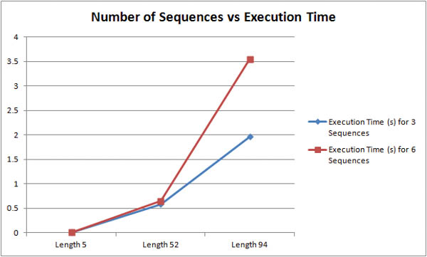
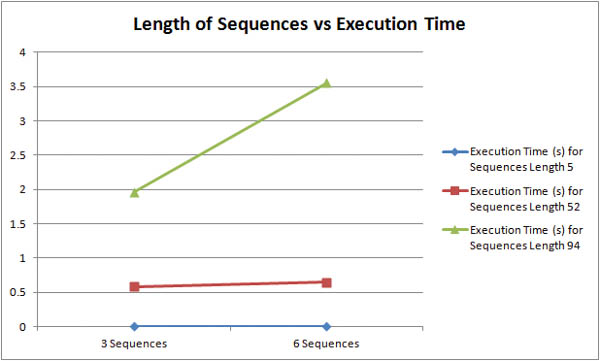
How does the length of input sequences affect the runtime of the algorithm? The graph above shows that longer sequences are much more computationally taxing than shorter sequences. For inputs of three sequences, roughly doubling the character length from 52 to 94 characters resulted in a 330% increase in execution time. For inputs of six sequences, roughly doubling the character length from 52 to 94 resulted in a 550% increase in execution time. The graph below shows more concisely that longer sequences are more expensive than more sequences.

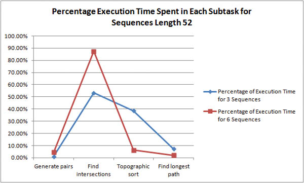
Where is the bottleneck in the algorithm? For shorter sequences, it is unclear whether pair generation or intersection discovery is the more time-expensive task.

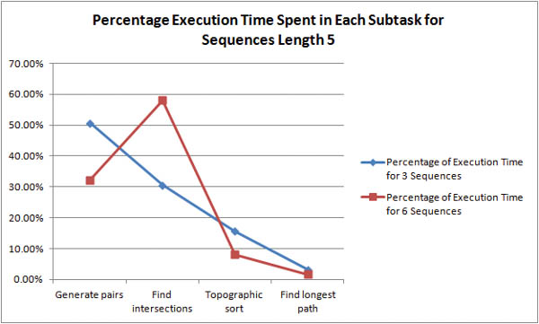
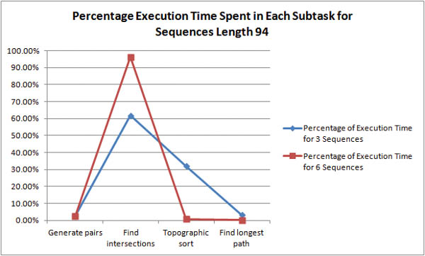
As the length of the sequences is increased it becomes obvious that intersection discovery is the most time-expensive task in the algorithm. For example, with 6 sequences of length 94, the algorithm spends 96% of its execution time in intersection discovery!

As stated above, the time complexity of intersection discovery is O(k2n) where k is the number of sequences and n is number of pairs in a sequence pair list. To make this analysis consistent with the graphs, the complexity should be defined in reference to the sequence size and not pair list size. Since there are (1/2)(n -1)n pairs for a sequence of length n, a consistent time complexity would be O(k2n2) where k is the number of sequences and n is the length of the sequences. Since n is usually much larger than k, this explains why it seems longer sequences are much more time-expensive than a greater number of sequences.